Home BlogsGetting Started with HNSWlib

Getting Started with HNSWlib

Engineering

November 25, 2024

Haziqa Sajid

Semantic search allows machines to understand language and yield better search results, which is essential in AI and data analytics. Once the language is represented as embeddings, the search can be performed using exact or approximate methods. Approximate Nearest Neighbor (ANN) search is a method used to quickly find points in a dataset that are closest to a given query point, unlike exact nearest neighbor search, which can be computationally expensive for high-dimensional data. ANN allows faster retrieval by providing results that are approximately close to the nearest neighbors.

One of the algorithms for Approximate Nearest Neighbor (ANN) search is HNSW (Hierarchical Navigable Small Worlds), implemented under HNSWlib, which will be the focus of today’s discussion. In this blog, we will:

Understand the HNSW algorithm.
Explore HNSWlib and its key features.
Set up HNSWlib, covering index building and search implementation.
Compare it with Milvus.

Understanding HNSW

Hierarchical Navigable Small Worlds (HNSW) is a graph-based data structure that allows efficient similarity searches, particularly in high-dimensional spaces, by building a multi-layered graph of “small world” networks. Introduced in 2016, HNSW addresses the scalability issues associated with traditional search methods like brute-force and tree-based searches. It is ideal for applications involving large datasets, such as recommendation systems, image recognition, and retrieval-augmented generation (RAG).

Why HNSW Matters

HNSW significantly enhances the performance of nearest-neighbor search in high-dimensional spaces. Combining the hierarchical structure with small-world navigability avoids the computational inefficiency of older methods, enabling it to perform well even with massive, complex datasets. To understand this better, let’s look at how it works now.

How HNSW Works

Hierarchical Layers: HNSW organizes data into a hierarchy of layers, where each layer contains nodes connected by edges. The top layers are sparser, allowing for broad “skips” across the graph, much like zooming out on a map to see only major highways between cities. Lower layers increase in density, providing finer detail and more connections between closer neighbors.
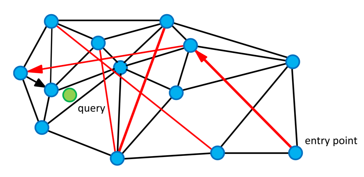
Navigable Small Worlds Concept: Each layer in HNSW builds on the concept of a “small world” network, where nodes (data points) are only a few “hops” away from each other. The search algorithm begins at the highest, sparsest layer and works downward, moving to progressively denser layers to refine the search. This approach is like moving from a global view down to neighborhood-level details, gradually narrowing the search area.

Fig 1: An Example of a Navigable Small World Graph

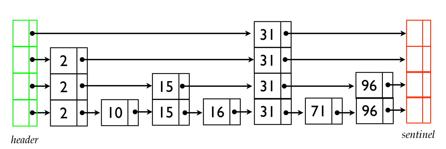
Skip List-Like Structure: The hierarchical aspect of HNSW resembles a skip list, a probabilistic data structure where higher layers have fewer nodes, allowing for faster initial searches.

Fig 2: An Example of Skip List Structure

To search for 96 in the given skip list, we begin at the top level on the far left at the header node. Moving to the right, we encounter 31, less than 96, so we continue to the next node. Now, we need to move down a level where we see 31 again; since it’s still less than 96, we descend another level. Finding 31 once more, we then move right and reach 96, our target value. Thus, we locate 96 without needing to descend to the lowest levels of the skip list.

Search Efficiency: The HNSW algorithm starts from an entry node at the highest layer, progressing to closer neighbors with each step. It descends through the layers, using each one for coarse-to-fine-grained exploration, until it reaches the lowest layer where the most similar nodes are likely found. This layered navigation reduces the number of nodes and edges that need to be explored, making the search fast and accurate.
Insertion and Maintenance: When adding a new node, the algorithm determines its entry layer based on probability and connects it to nearby nodes using a neighbor selection heuristic. The heuristic aims to optimize connectivity, creating links that improve navigability while balancing graph density. This approach keeps the structure robust and adaptable to new data points.

While we have a foundational understanding of the HNSW algorithm, implementing it from scratch can be overwhelming. Fortunately, the community has developed libraries like HNSWlib to simplify usage, making it accessible without scratching your head. So, let’s take a closer look at HNSWlib.

Overview of HNSWlib

HNSWlib, a popular library implementing HNSW, is highly efficient and scalable, performing well even with millions of points. It achieves sublinear time complexity by allowing quick jumps between graph layers and optimizing the search for dense, high-dimensional data. Here are the key features of HNSWlib include:

Graph-Based Structure: A multi-layered graph represents data points, allowing fast, nearest-neighbor searches.
High-Dimensional Efficiency: Optimized for high-dimensional data, providing quick and accurate approximate searches.
Sublinear Search Time: Achieves sublinear complexity by skipping layers, improving speed significantly.
Dynamic Updates: Supports real-time insertion and deletion of nodes without requiring a complete graph rebuild.
Memory Efficiency: Efficient memory usage, suitable for large datasets.
Scalability: Scales well to millions of data points, making it ideal for medium-scale applications like recommendation systems.

Note: HNSWlib is excellent for creating simple prototypes for vector search applications. However, due to scalability limitations, there may be better choices such as purpose-built vector databases for more complex scenarios involving hundreds of millions or even billions of data points. Let’s see that in action.

Getting Started with HNSWlib: A Step-by-Step Guide

This section will demonstrate using HNSWlib as a vector search library by creating an HNSW index, inserting data, and performing searches. Let’s start with installation:

Setup and Imports

To get started with HNSWlib in Python, first install it using pip:

pip install hnswlib

Then, import the necessary libraries:

import hnswlib 
import numpy as np

Preparing Data

In this example, we’ll use NumPyto generate a random dataset with 10,000 elements, each with a dimension size 256.

dim = 256  # Dimensionality of your vectors
num_elements = 10000  # Number of elements to insert

Let’s create the data:

data = np.random.rand(num_elements, dim).astype(np.float32)  # Example data

Now our data is ready, let’s build an index.

Building an Index

In building an index, we need to define the dimensionality of the vectors and the space type. Let’s create an index:

p = hnswlib.Index(space='l2', dim=dim)

space='l2': This parameter defines the distance metric used for similarity. Setting it to 'l2' means using the Euclidean distance (L2 norm). If you instead set it to 'ip', it would use the inner product, which is helpful for tasks like cosine similarity.

dim=dim: This parameter specifies the dimensionality of the data points you’ll be working with. It must match the dimension of the data you plan to add to the index.

Here’s how to initialize an index:

p.init_index(max_elements=num_elements, ef_construction=200, M=16)

max_elements=num_elements: This sets the maximum number of elements that can be added to the index. Num_elements is the maximum capacity, so we set this to 10,000 as we are working with 10,000 data points.

ef_construction=200: This parameter controls the accuracy vs. construction speed trade-off during index creation. A higher value improves recall (accuracy) but increases memory usage and build time. Common values range from 100 to 200.

M=16: This parameter determines the number of bi-directional links created for each data point, influencing accuracy and search speed. Typical values are between 12 and 48; 16 is often a good balance for moderate accuracy and speed.

p.set_ef(50)  # This parameter controls the speed/accuracy trade-off

ef: The ef parameter, short for “exploration factor,” determines how many neighbors are examined during a search. A higher ef value results in more neighbors being explored, which generally increases the accuracy (recall) of the search but also makes it slower. Conversely, a lower ef value can search faster but might reduce accuracy.

In this case, Setting ef to 50 means the search algorithm will evaluate up to 50 neighbors when finding the most similar data points.

Note: ef_construction sets neighbor search effort during index creation, enhancing accuracy but slowing construction. ef controls search effort during querying, balancing speed and recall dynamically for each query.

Performing Searches

To perform a nearest neighbor search using HNSWlib, we first create a random query vector. In this example, the vector’s dimensionality matches the indexed data.

query_vector = np.random.rand(dim).astype(np.float32)  # Example query

labels, distances = p.knn_query(query_vector, k=5)  # k is the number of nearest neighbors

query_vector: This line generates a random vector with the same dimensionality as the indexed data, ensuring compatibility for the nearest neighbor search.
knn_query: The method searches for the k nearest neighbors of the query_vector within the index p. It returns two arrays: labels, which contain the indices of the nearest neighbors, and distances, which indicate the distances from the query vector to each of these neighbors. Here, k=5 specifies that we want to find the five closest neighbors.

Here are the results after printing the labels and distances:

print("Nearest neighbors' labels:", labels)
print("Distances:", distances)

> Nearest neighbors' labels: [[4498 1751 5647 4483 2471]]
> Distances: [[33.718    35.484592 35.627766 35.828312 35.91495 ]]

Here we have it, a simple guide to get your wheels started with HNSWlib.

As mentioned, HNSWlib is a great vector search engine for prototyping or experimenting with medium-sized datasets. If you have higher scalability requirements or need other enterprise-level features, you may need to choose a purpose-built vector database like the open-source Milvus or its fully managed service on Zilliz Cloud. So, in the following section, we will compare HNSWlib with Milvus.

HNSWlib vs. Purpose-Built Vector Databases Like Milvus

A vector database stores data as mathematical representations, enabling machine learning models to power search, recommendations, and text generation by identifying data through similarity metrics for contextual understanding.

Vector indices libraries like HNSWlib improve vector search and retrieval but lack the management features of a full database. On the other hand, vector databases, like Milvus, are designed to handle vector embeddings at scale, providing advantages in data management, indexing, and querying capabilities that standalone libraries typically lack. Here are some other benefits of using Milvus:

High-Speed Vector Similarity Search: Milvus provides millisecond-level search performance across billion-scale vector datasets, ideal for applications like image retrieval, recommendation systems, natural language processing (NLP), and retrieval augmented generation (RAG).
Scalability and High Availability: Built to handle massive data volumes, Milvus scales horizontally and includes replication and failover mechanisms for reliability.
Distributed Architecture: Milvus uses a distributed, scalable architecture that separates storage and computing across multiple nodes for flexibility and robustness.
Hybrid search: Milvus supports multimodal search, hybrid sparse and dense search, and hybrid dense and full-text search, offering versatile and flexible search functionality.
Flexible Data Support: Milvus supports various data types—vectors, scalars, and structured data—allowing seamless management and analysis within a single system.
Active Community and Support: A thriving community provides regular updates, tutorials, and support, ensuring Milvus remains aligned with user needs and advances in the field.
AI integration: Milvus has integrated with various popular AI frameworks and technologies, making it easier for developers to build applications with their familiar tech stacks.

Milvus also provides a fully managed service on Ziliz Cloud, which is hassle-free and 10x faster than Milvus.

Comparison: Milvus vs. HNSWlib

Feature	Milvus	HNSWlib
Scalability	Handles billions of vectors with ease	Fit for smaller datasets due to RAM usage
Ideal for	Prototyping, experimenting, and enterprise-level applications	Focuses on prototypes and lightweight ANN tasks
Indexing	Supports 10+ indexing algorithms, including HNSW, DiskANN, Quantization, and Binary	Uses a graph-based HNSW only
Integration	Offers APIs and cloud-native services	Serves as a lightweight, standalone library
Performance	Optimizes for large data, distributed queries	Offers high speed but limited scalability

Overall, Milvus is generally preferable for large-scale, production-grade applications with complex indexing needs, while HNSWlib is ideal for prototyping and more straightforward use cases.

Conclusion

Semantic search can be resource-intensive, so internal data structuring, like that performed by HNSW, is essential for faster data retrieval. Libraries like HNSWlib care about the implementation, so the developers have the recipes ready to prototype vector capabilities. With just a few lines of code, we can build up our own index and perform searches.

HNSWlib is a great way to start. However, if you want to build complex and production-ready AI applications, purpose-built vector databases are the best option. For example, Milvus is an open-source vector database with many enterprise-ready features such as high-speed vector search, scalability, availability, and flexibility in terms of data types and programming language.