Understanding Hierarchical Navigable Small Worlds (HNSW) for Vector Search

The key operation of vector databases is similarity search, which involves finding the nearest neighbors in the database to a query vector, for example, by Euclidean distance. A naive method would calculate the distance from the query vector to every vector stored in the database and take the top-K closest. However, this clearly does not scale as the size of the database grows. In practice, a naive similarity search is practical only for databases with fewer than around 1 million vectors. How are we to scale our search to the 10s and 100s of millions, or even to the billions of vectors?

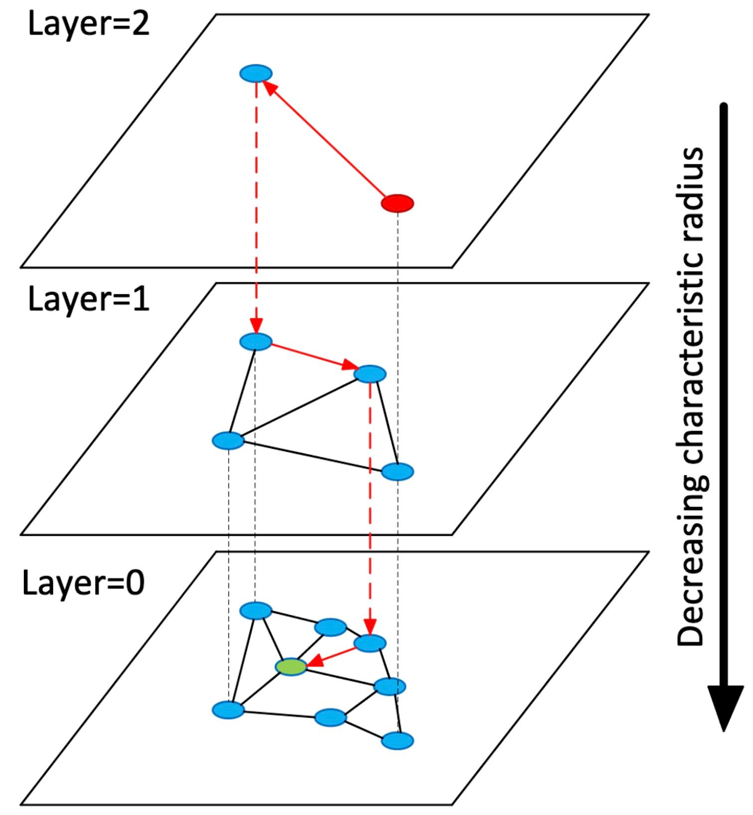
Figure: Descending a hierarchy of vector search indices

Many algorithms and data structures have been developed to scale similarity search in high-dimensional vector spaces to sub-linear time complexity. In this article, we’ll explain and implement a popular and effective method called Hierarchical Navigable Small Worlds (HNSW), which is frequently the default choice for medium-sized vector datasets. It belongs to the family of search methods that construct a graph over the vectors, where vertices denote vectors and edges denote similarity between them. Search is performed by navigating the graph, in the simplest case, greedily traversing to the neighbor of the current node that is closest to the query and repeating until a local minimum is reached.

We will explain in more detail how the search graph is constructed, how the graph enables search, and at the end, link to an HNSW implementation, by yours truly, in simple Python.

Navigable Small Worlds

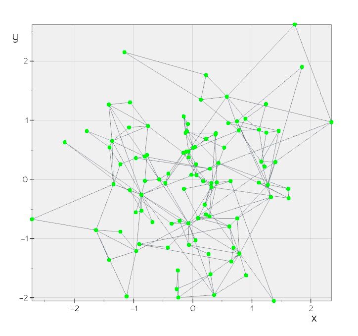
Figure: NSW graph created from 100 randomly located 2D points.

As mentioned, HNSW constructs a search graph offline before we can perform a query. The algorithm builds on top of prior work, a method called Navigable Small Worlds (NSW). We will explain NSW first and it will then be trivial to go from there to Hierarchical NSW. The illustration above is of a constructed search graph for NSW over 2-dimensional vectors. In all examples below, we restrict ourselves to 2-dimensional vectors so as to be able to visualize them.

Constructing the Graph

An NSW is a graph where the vertices represent vectors and the edges are constructed heuristically from the similarity between vectors so that most vectors are reachable from anywhere via a small number of hops. This is the so-called “small world” property that permits quick navigation. See the above figure.

The graph is initialized to be empty. We iterate through the vectors, adding each to the graph in turn. For each vector, starting at a random entry node, we greedily find the closest R nodes reachable from the entry point in the graph so far constructed. These R nodes are then connected to a new node representing the vector being inserted, optionally pruning any neighboring nodes that now have more than R neighbors. Repeating this process for all vectors will result in the NSW graph. See the above illustration visualizing the algorithm, and refer to the resources at the end of the article for a theoretical analysis of the properties of a graph constructed like this.

Searching the Graph

We have already seen the search algorithm from its use in graph construction. In this case, however, the query node is provided by the user, rather than being one for insertion into the graph. Starting from a random entry note, we greedily navigate to its neighbor closest to the query, maintaining a dynamic set of the closest vectors encountered so far. See the illustration above. Note that we can enhance search accuracy by initiating searches from multiple random entry points and aggregating the results, along with considering multiple neighbors at each step. However, these improvements come at the cost of increased latency.

So far, we have described the NSW algorithm and data structure that can help us scale up search in high-dimensional space. Nonetheless, the method suffers serious shortcomings, including failure in low dimensions, slow search convergence, and a tendency to be trapped in local minima.

The authors of HNSW fix these shortcomings with three modifications to NSW:

• Explicit selection of the entry nodes during construction and search;

• Separation of edges by different scales; and,

• Use of an advanced heuristic to select the neighbors.

The first two are realized with a simple idea: building a hierarchy of search graphs. Instead of a single graph, as in NSW, HNSW constructs a hierarchy of graphs. Each graph, or layer, is individually searched in the same way as NSW. The top layer, which is searched first, contains very few nodes, and deeper layers progressively include more and more nodes, with the bottom layer including all nodes. This means that the top layers contain longer hops across the vector space, permitting a sort of course-to-fine search. See above for an illustration.

Constructing the Graph

The construction algorithm works as follows: we fix a number of layers, L, in advance. The value l=1 will correspond to the coarsest layer, where search begins, and l=L will correspond to the densest layer, where search finishes. We iterate through each vector to be inserted and sample an insertion layer following a truncated geometric distribution (either rejecting l > L or setting l’ = min_(l, L)_). Say we sample 1 < l < L for the current vector. We perform a greedy search on the top layer, L, until we reach its local minimum. Then, we follow an edge from the local minimum in the _L_th layer to the corresponding vector in the _(L-1)_th layer and use it as the entry point to greedily search the _(L-1)_th layer.

This process is repeated until we reach the _l_th layer. We then begin to create nodes for the vector to be inserted, connecting it to its closest neighbors found by greedy search in the _l_th layer so far constructed, navigating to the _(l-1)_th layer and repeating until we have inserted the vector into the _1_st layer. An animation above makes this clear

We can see that this hierarchical graph construction method uses a clever explicit selection of the insertion node for each vector. We search the layers above the insertion layer constructed so far, searching efficiently from course-to-fine distances. Relatedly, the method separates links by different scales in each layer: the top layer affords long-scale hops across the search space, with the scale diminishing down to the bottom layer. Both of these modifications help avoid being trapped in sub-optimal minima and hasten search convergence at the cost of additional memory.

Searching the Graph

The search procedure works much like the inner graph construction step. Starting from the top layer, we greedily navigate to the node or nodes closest to the query. Then we follow that node(s) down to the next layer and repeat the process. Our answer is obtained by the list of R closest neighbors in the bottom layer, as illustrated by the animation above this.

Conclusion

Vector databases like Milvus provide highly optimized and tuned implementations of HNSW, and it is often the best default search index for datasets that fit in memory.

We have sketched a high-level overview of how and why HNSW works, preferring visualizations and intuition over theory and mathematics. Consequently, we have omitted an exact description of the construction and search algorithms[Malkov and Yashushin, 2016; Alg 1-3], analysis of search and construction complexity [Malkov and Yashushin, 2016; §4.2], and less essential details like a heuristic for more effectively choosing neighbor nodes during construction [Malkov and Yashushin, 2016; Alg 5]. Moreover, we have omitted discussion of the algorithm’s hyperparameters, their meaning and how they affect the latency/speed/memory trade-off [Malkov and Yashushin, 2016; §4.1]. An understanding of this is important for using HNSW in practice.

The resources below contain further reading on these topics and a full Python pedagogical implementation (written by myself) for NSW and HNSW, including code to produce the animations in this article.

• GitHub: “HNSW-Illustrated: A small implementation of Hierarchical Navigable Small Worlds (HNSW), a vector search algorithm, for learning purposes”

• HNSW

• Understanding Hierarchical Navigable Small Worlds (HNSW) - Zilliz Learn

• HNSW paper: “Efficient and robust approximate nearest neighbor search using Hierarchical Navigable Small World graphs”

• NSW paper: “Approximate nearest neighbor algorithm based on navigable small world graphs”