

Embedding-based diversity sampling picks examples that are spread out in embedding space instead of drawing uniformly at random, so a labeling or training budget covers many kinds of data rather than repeating the densest region. The usual recipes are cluster-then-sample (k-means strata with a per-cluster cap), greedy farthest-point or k-center selection (the “core-set” approach from active learning), and near-duplicate suppression before sampling. A vector database such as Milvus makes these practical at scale because the core operation in every recipe is the same: given a point, find its neighbors, or how far it is from everything already selected.
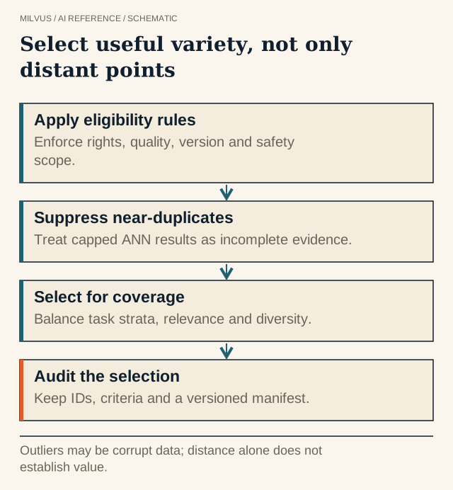 Select useful variety, not only distant points. Outliers may be corrupt data; distance alone does not establish value.
Why random sampling under-covers real datasets
Real corpora are lopsided. A driving dataset is mostly highway frames, a support-ticket archive is mostly password resets, and a scraped web corpus repeats the same boilerplate thousands of times. Uniform random sampling preserves that skew: if 70% of the data is one scene, roughly 70% of the labeling budget goes to it, and the rare cases that limit model quality get a handful of examples or none.
Embeddings let you see that structure. Items that look or read alike sit close together, so density in embedding space is a proxy for redundancy. Sampling for spread rather than frequency gives each region of the space a fair share of the budget. Active-learning research (Sener and Savarese’s core-set formulation, and later density-aware variants such as ProbCover) showed that labeling a well-spread subset can match or beat random selection at the same budget, and data-pruning work on large image-text corpora (SemDeDup) showed that removing semantically redundant examples can cut training data substantially with little accuracy loss.
Which embedding sampling method fits your goal?
| Method | How it works | Best for | Main risk |
|---|---|---|---|
| Stratified by cluster | k-means on embeddings, then sample up to n per cluster | Balancing topics or scenes in a training mix | Cluster count sets the granularity; tiny clusters may be noise |
| k-center greedy (core-set) | Repeatedly add the point farthest from everything selected | Small labeling budgets that must cover the whole space | Pulls in outliers, corrupted files, and junk first |
| Density-weighted | Prefer points in well-populated but under-sampled regions | Avoiding the outlier bias of pure k-center | Needs a neighborhood-density estimate |
| Dedup then random | Remove near-duplicates by similarity threshold, then sample | Web-scale corpora with heavy repetition | Threshold too loose removes real variants |
| Query-driven coverage | Search with seed queries for each required scenario | Guaranteeing must-have cases are present | Only finds what you thought to ask for |
Most production pipelines combine two of these: deduplicate first, then stratify, then top up rare-but-required scenarios with targeted searches.
How to run diversity sampling with Milvus
Assume the candidate pool is in a collection with a FLOAT_VECTOR field, a primary key, and scalar metadata such as source, language, or scene_type.
Step 1: suppress near-duplicates with range search
For each candidate, a range search returns neighbors above a similarity threshold, up to limit and subject to the same ANN approximation as any search. It is a near-duplicate detector, not a full census: if a query returns exactly limit hits, the true group is probably larger. With the COSINE metric, radius is the exclusive lower bound and range_filter the inclusive upper bound:
res = client.search(
    collection_name="pool",
    data=[candidate_vec],
    limit=100,
    search_params={"metric_type": "COSINE", "params": {"radius": 0.95, "range_filter": 1.0}},
    output_fields=["id", "quality_score"],
)
Keep the highest-quality member of each tight group and mark the rest sample_status = "redundant". Calibrate the 0.95 on labeled pairs from your own data; the right value depends on the model. The deduplication guide covers that calibration.
Step 2: stratify by cluster
Export vectors and run k-means outside the database, then write cluster_id back as an INT64 scalar field (see document clustering with embeddings). With a scalar index on cluster_id, drawing a capped sample per stratum is a filtered query:
rows = client.query(
    collection_name="pool",
    filter='cluster_id == 42 and sample_status == "candidate"',
    output_fields=["id", "quality_score"],
    limit=200,
)
Choose the per-cluster cap deliberately. Equal allocation over-weights tiny clusters; proportional allocation reproduces the original skew. A square-root allocation, or a cap plus a minimum, is a common middle ground.
Step 3: greedy farthest-point selection with an “already selected” collection
For k-center selection, keep the chosen examples in a second small collection. For each candidate, search the selected collection with limit=1; the distance to the nearest selected item is its novelty score. Add the candidate with the largest score, insert it into the selected collection, and repeat. On a large pool, evaluate candidates in batches (Milvus accepts many query vectors per search call) and add the top few per round rather than one at a time. Because every round is an ANN lookup against a small collection, this scales to pools that would be impractical with an in-memory pairwise distance matrix.
To avoid k-center’s appetite for junk, gate candidates with a quality filter first (quality_score > 0.5, a valid decode flag, a language check) and down-weight points that have no neighbors at all within a modest radius, since an isolated vector is as likely to be a corrupt file as a valuable edge case.
Step 4: guarantee required scenarios
Coverage targets such as “at least 500 night-time rain frames” or “every supported language” should not depend on geometry. Use seed text or example vectors per scenario, run a filtered search (filter='language == "ko"'), and add the results until each target is met. Metadata filters handle the properties embeddings do not encode well, such as license, geography, or label availability. How filters interact with vector search explains the performance side.
Don’t confuse IVF centroids with sampling strata
IVF_FLAT and related indexes also run k-means (nlist clusters, 128 by default), but those centroids are built per segment to speed up search and are not returned to applications. Compute your own clusters for sampling and store them as fields; that also lets you pick a granularity that suits the dataset rather than the index.
How do you know the sample is more diverse and more useful?
Measure both sides. Diversity metrics include the number of clusters covered, the entropy of the cluster distribution, the average nearest-neighbor distance within the sample, and the duplicate rate. Usefulness metrics come from the downstream task: label yield, model accuracy on rare-slice test sets, and retrieval quality on held-out queries. Always compare against a random sample of the same size; a sample that is beautifully spread but full of noise is a regression.
Record the embedding model, cluster run, thresholds, and the reason each item was selected (stratum, novelty, required_scenario) as fields or in a manifest, so the selection can be reproduced. When the embedding model changes, the geometry changes, and both clusters and novelty scores must be recomputed. The guide to reproducible vector-search and training experiments covers versioning those inputs.
Next step
Load a candidate pool into Milvus with the Quickstart, then try range-search dedup and a capped per-cluster query on it. For curation workflows that combine these steps, see what data curation looks like with vector search and how to select rollouts for offline training.
Sources and further reading
- Sener and Savarese, Active Learning for Convolutional Neural Networks: A Core-Set Approach (arXiv)
- Abbas et al., SemDeDup: Data-efficient learning at web-scale through semantic deduplication (arXiv)
- Sentence Transformers: embedding-based clustering
- Milvus range search
- Milvus IVF_FLAT index
- Milvus scalar queries and iterators


