Hyperbolic Search on Zilliz Cloud

This is part 3 of a four-part series on hyperbolic embeddings in vector search: how to search them in Milvus and Zilliz Cloud with plain inner product, and when they’re worth using. This post measures recall, capacity and latency on Zilliz Cloud. Part 1 explains why plain inner product works, part 2 runs it on Milvus, and part 4 compares a hyperbolic model with CLIP.

A quick recap from part 1. Each hyperbolic embedding is 513 numbers on a bowl-shaped surface, the Lorentz hyperboloid. The first number is the point’s height up the bowl,^[1] which rises with its radius, the distance from the center:

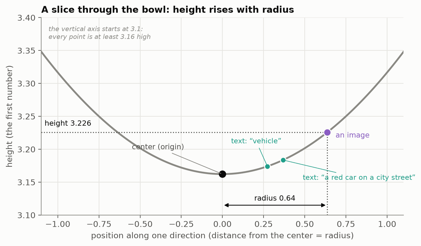The curve is the bowl seen side-on: move away from the center in any direction (horizontal axis) and the height, the first number, rises (vertical axis). The vertical axis starts at 3.1, which exaggerates the curve; every point is at least 3.16 high, which is why raw heights all sit around 3.2.

Hyperbolic search then runs on any database that offers plain, unnormalized inner-product search. Flip the sign of the query’s height, and the database’s top results are exactly the hyperbolic top results. Subtract the corpus average height from every stored document (centering), and the vectors index well, with no rerank. On self-hosted Milvus, that let HNSW reach a recall@10 of 0.996 (part 2).

This post asks what the same vectors do on a managed service: about 1.28 million ImageNet images,^[2] embedded as 513-dimensional vectors by Hyper3-CLIP V1 (hyper3labs/hyper3-clip-v1). How much recall, how much capacity, and how fast?

In short: centered, a single search reaches a recall@10 of about 0.98 in about 4 ms; a shortlist and rerank reaches 0.999 for a little more latency; and a 1 CU cluster holds at least 2.8 million of these vectors.

A managed index

On Zilliz Cloud you don’t pick an index type or tune HNSW’s ef or IVF’s nprobe. The service chooses and manages the index for you (AUTOINDEX), and exposes a single search level from 1 to 10: higher levels search harder, for better recall at some cost in latency. You also choose a build level when the index is built, which trades storage capacity against precision (Tune Index Build Level).

We used the precision-first build (build_level=2) on a Performance-optimized Dedicated cluster in aws-eu-west-1. Using Strategy A from part 2 (one 513-number vector per image, searched by inner product), we loaded the raw and centered vectors side by side and asked each for its top 10 at level=10. We also asked for wider shortlists, and checked how many of the true top 10 each shortlist contained, since a shortlist is what a reranking step would work from. Each ± is a 95% confidence interval.

	raw	centered	gain
recall@10	0.853 ± 0.010	0.982 ± 0.003	+0.130
true top 10 found in a 50-result shortlist	0.881 ± 0.009	0.991 ± 0.003	+0.110
… in a 200-result shortlist	0.923 ± 0.007	0.996 ± 0.002	+0.072
… in a 1,000-result shortlist	0.980 ± 0.004	over 0.999	+0.020

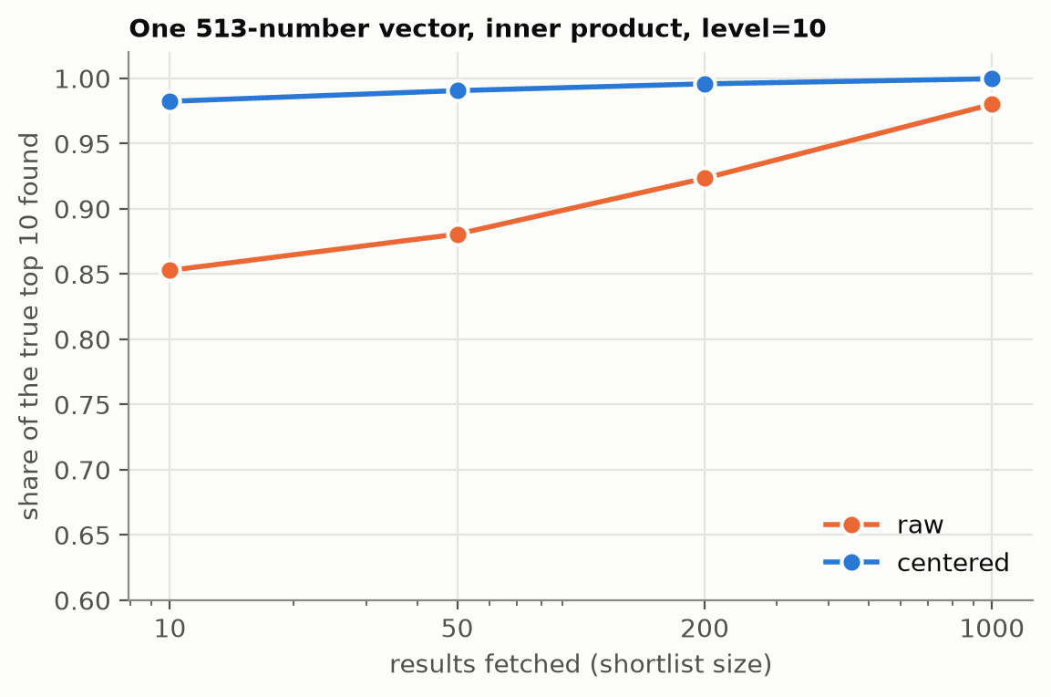Further right is a bigger shortlist (log scale); higher means more of the true top 10 inside it. Centered (blue) starts near the top with a plain 10-result search; raw (orange) needs a 1,000-result shortlist, and a rerank, to come close.

Centering matters as much on a managed index as on self-hosted Milvus. Raw, the service misses 0.147 of the true top 10; centered, it misses 0.018. That is 88% fewer misses, and centered vectors reach a recall@10 of 0.982 in a single request. Centered, a 10-result search already matches what raw vectors manage with a 1,000-result shortlist.

The scores the service returns are accurate too. Once the constant offset from centering is removed, they are typically within 0.000011 of the exact Lorentz score, about ten times smaller than the typical gap between the 10th and 11th results, so the order survives.

Capacity

We chose the precision-first build on a performance-optimized cluster type, which trades data density for optimal recall and latency. Zilliz Cloud clusters are sized in CUs (compute units, the service’s unit of cluster capacity). On a fresh 1 CU Performance-optimized cluster holding only the centered collection, the 1.28 million embeddings consumed 34.2% of the cluster capacity.

Keeping to an 80% watermark (a safety margin that leaves headroom for growth and background work), that gives at least 2.8 million embeddings per CU. The pricing calculator turns that into a monthly cost for your region and corpus size.

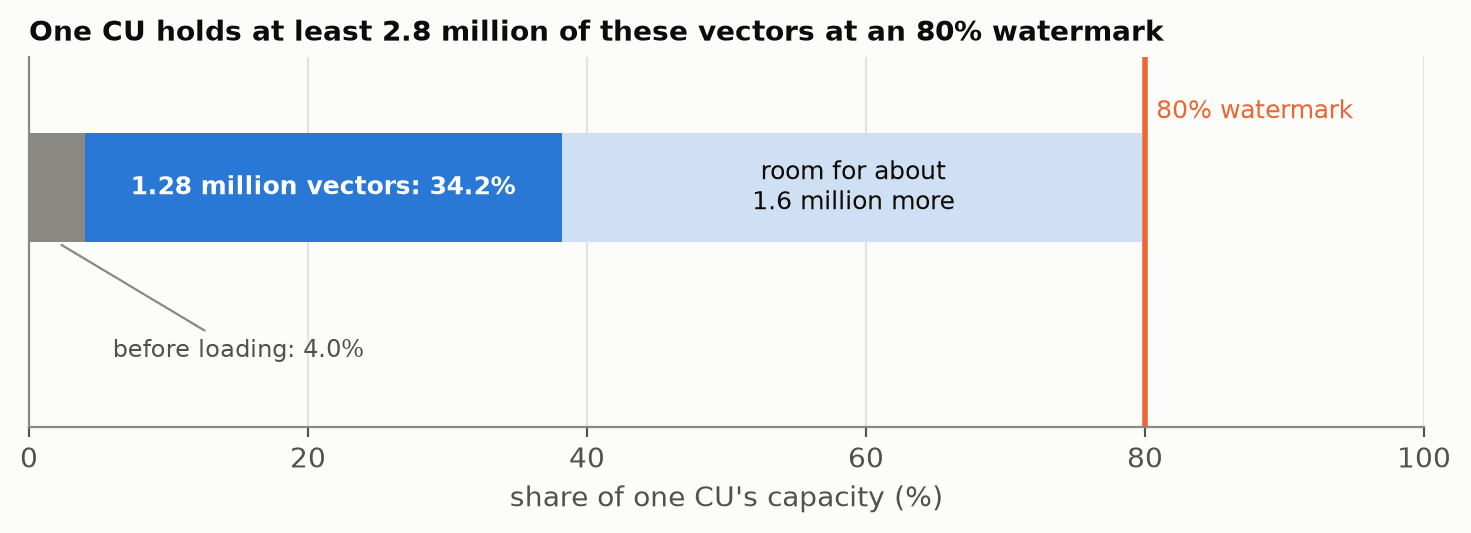One CU drawn as a bar from 0 to 100%. Gray is the empty cluster's overhead, dark blue our 1.28 million vectors, and pale blue the headroom left before the 80% watermark (orange line).

Larger data sets will benefit from optimization at scale, so treat this as a conservative minimum capacity. Additional fields and indexes will consume a small amount of capacity as well, so we always recommend deploying a proof-of-concept cluster to measure the real capacity for your requirements.

Latency

We ran the benchmark from a c7i.large EC2 instance (a small AWS virtual machine) in eu-west-1a, the same AWS region as the cluster. That matters more than any tuning. Just opening a connection takes 1.48 ms in-region (median), against 15.04 ms from a laptop in the UK: ten times longer before any search runs. From the laptop, every configuration measured 16 to 17 ms and looked the same.

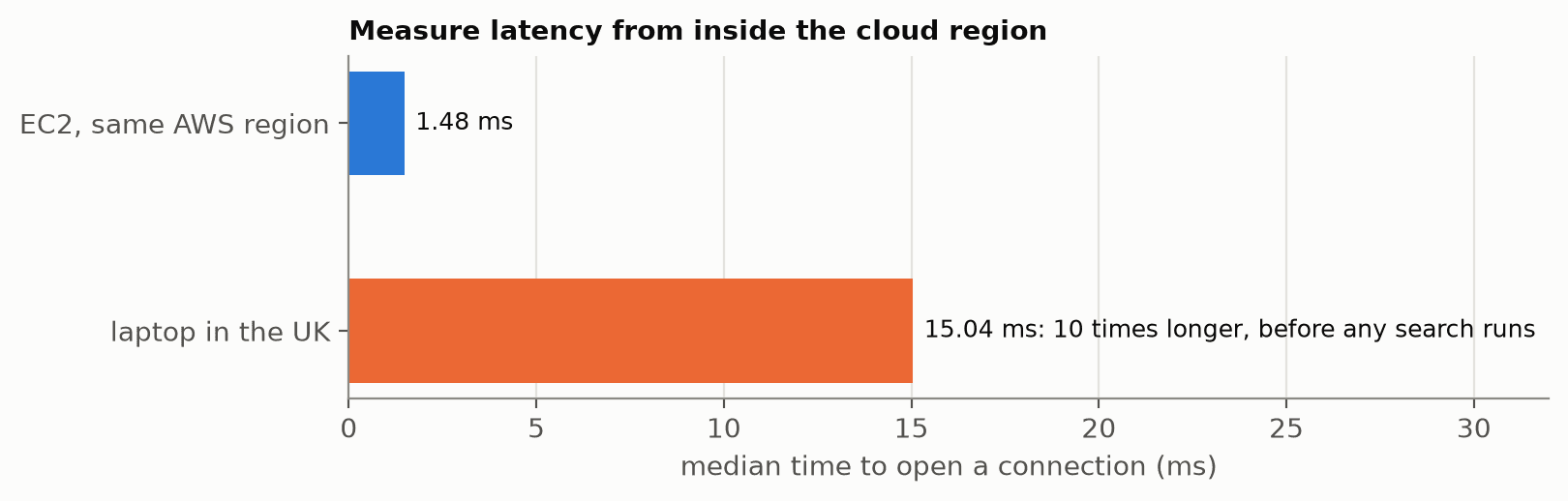Shorter is better. From the laptop, opening a connection alone takes longer than any search we measured, enough to hide the differences between configurations, so we benchmarked in-region.

We compared centered Strategy A with Strategy B from part 2, which stores the 512-number direction plus the height and radius as scalar fields, fetches candidates with a cosine search, and reranks them exactly. Cosine alone finds only 0.745 of the true top 10, because it ignores how far each item sits from the center, but 200 candidates hold over 0.999 of them, so the rerank recovers almost the whole true top 10.

The figures below are in-region: 500 prompts, top 10, 3 repeats, with the first 50 queries discarded as warm-up. Every collection uses the precision-first build, and every configuration ran in the same session. p50 is the median latency; QPS is queries per second, and peak QPS the highest throughput we measured. Medians moved from one run to the next, so we ran each configuration four times at one query at a time: p50 is the median of those four runs, and recall and peak QPS come from the first.

config	recall@10	p50	peak QPS
A centered, level=10	0.977	3.75 ms	1,698
A centered, level=5	0.888	3.26 ms	2,345
B, 200 candidates, level=1	0.995	4.37 ms	1,314
B, 1,000 candidates, level=1	0.999	6.61 ms	384

The two designs trade recall against speed. Centered A at level=10 reaches a recall@10 of 0.977 at 3.75 ms, with the highest throughput of any configuration above 0.9 recall, and it was the steadiest: its median moved only between 3.67 and 3.80 ms across the four runs. B with 200 candidates finds more, 0.995, at 4.37 ms, but less steadily: its median ranged from 3.80 to 5.19 ms, and its peak throughput is 23% lower. Raising B’s level to 10 lifts it to 0.999 for about 0.9 ms more at the median; 1,000 candidates also gives 0.999, for about 2.2 ms more. The rerank itself is cheap: in-region, it took 0.15 ms over 200 candidates and 0.51 ms over 1,000.

Rerank inside Zilliz Cloud

Strategy B’s rerank can also run in the database, as a function chain (part 2 has the code). Your application then sends one request and gets back the hyperbolic top 10, with no rerank code of its own. We tested function chains on Milvus 3.0.1, so ensure your Zilliz deployment is running 3.0.1 or later.

We measured it in the same session, on the same collection, against B with the rerank in the application, both at level=10:

config	recall@10	p50	peak QPS
B, rerank in the application, 200 candidates	0.999	5.27 ms	1,211
B, rerank in the database, 200 candidates	0.999	4.70 ms	1,124
B, rerank in the application, 1,000 candidates	0.999	8.05 ms	370
B, rerank in the database, 1,000 candidates	over 0.999	6.47 ms	660

Both ways return the same results: the same top 10 for 499 of 500 queries at 200 candidates, and 497 of 500 at 1,000. With 200 candidates, the two are close. The rerank in the database had the lower median, 4.70 ms against 5.27 ms, but the medians overlapped from run to run (4.63 to 5.64 ms in the database, 4.67 to 6.10 ms in the application), and its peak throughput was 7% lower. With 1,000 candidates, where the application would otherwise receive and rerank 1,000 results per query, the rerank in the database was faster in every run (6.41 to 7.39 ms against 7.67 to 8.89 ms), with 1.8 times the peak throughput.

This depends on the level, in a way we haven’t explained. At level=1, the rerank in the database was slower in every run, by about 1.1 ms at the median with 200 candidates and 1.6 ms with 1,000. Within the database, latency was lowest at level=5 with 200 candidates (4.11 ms) and highest there with 1,000 (10.14 ms), in every run. Try a few levels on your own cluster.

Against a plain cosine index

What does hyperbolic search cost compared with a conventional setup? We loaded 1.28 million CLIP ViT-B/16^[3] image vectors (512-dimensional, searched with cosine, same precision-first build) onto the same cluster. We timed them in the same run as centered Strategy A, using real CLIP text queries. Each model’s recall is measured against its own exact top 10.

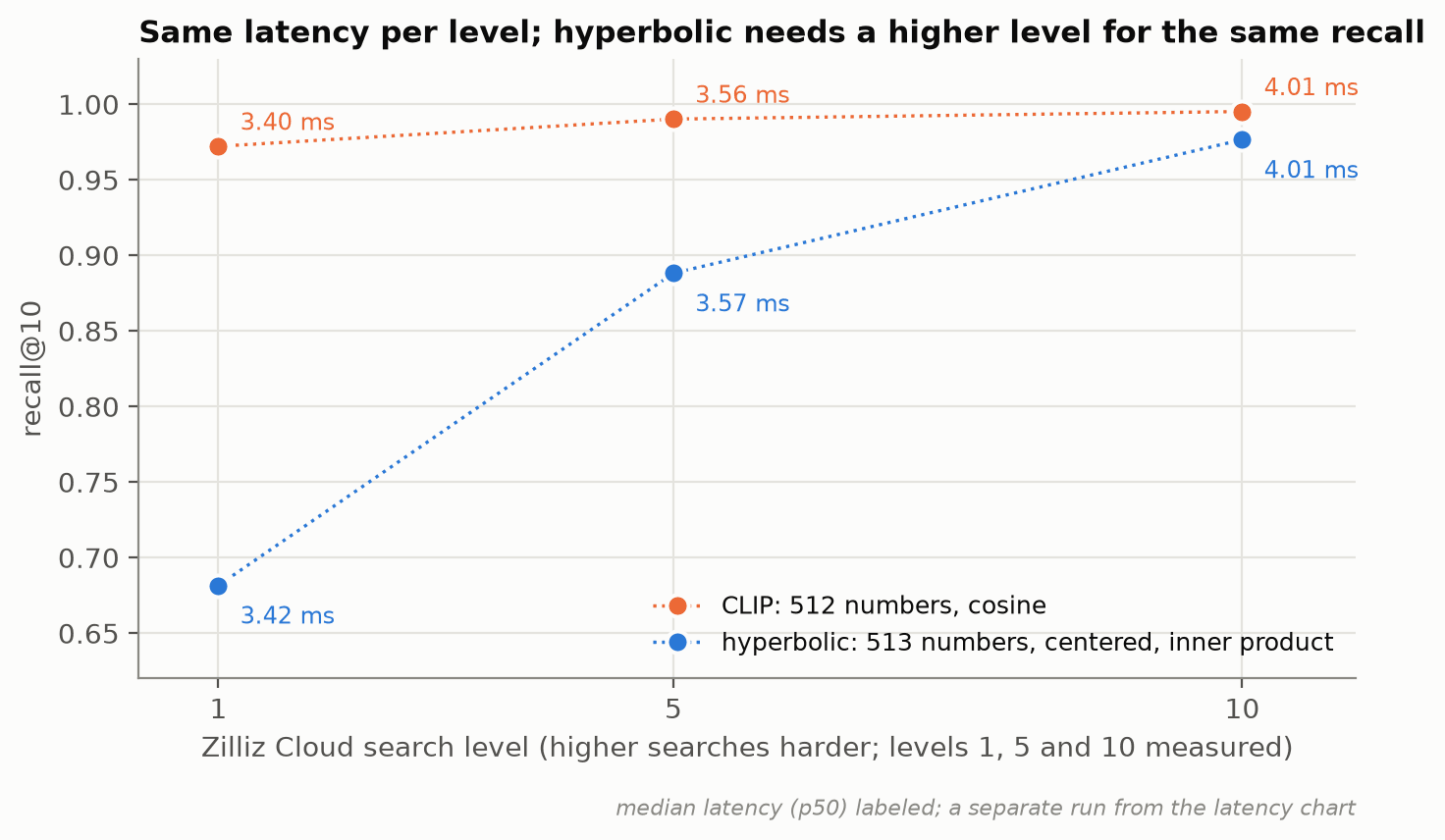Each line follows one model as the search level rises (left to right); height is recall, and the label by each dot is its median latency. The latencies match at every level, so a search costs the same for both. The hyperbolic line starts lower and needs level 10 to approach CLIP.

level	hyperbolic, A centered	p50	CLIP, cosine	p50
1	0.682	3.42 ms	0.972	3.40 ms
5	0.888	3.57 ms	0.990	3.56 ms
10	0.977	4.01 ms	0.995	4.01 ms

At the same level, a search costs the same: a 513-dimensional inner product is no slower than a 512-dimensional cosine. The difference is how hard the vectors are to navigate. CLIP reaches a recall@10 of 0.972 at level=1; the centered hyperbolic vectors need level=10 for the same recall.

Hyperbolic vectors aren’t always the harder ones to navigate. HypRAG’s authors^[4] indexed their text model, HyTE-FH, and a flat baseline, EucBERT, with Faiss’s HNSW, and report that the sign-flipped hyperbolic vectors were found more reliably (recall@10 0.906 against 0.891) and faster. They don’t center, and we haven’t measured centering on their vectors. Their models, data and index differ from ours, so the two results don’t conflict: how easy vectors are to navigate depends on the model that made them. Measure yours.

Takeaway

• Centering is essential on the managed index too. Without it, Zilliz Cloud misses more than one true neighbor in seven; with it, the service reaches a recall@10 of 0.982 in one request, with no rerank, in about 4 ms a search.
• Capacity is predictable. A 1 CU cluster holds at least 2.8 million of these 513-dimensional vectors at an 80% watermark.
• What hyperbolic costs. Against a plain CLIP cosine index on the same cluster, each search at a given level costs the same. Matching CLIP’s recall costs 0.61 ms more at the median and 23% lower peak throughput (still over 2,000 QPS on the small test cluster).

Which design to deploy depends on what you need most. Use the precision-first build for either, and center the documents for Strategy A.

Goal	Design	Setting	recall@10
simplest; lowest, steadiest latency; highest throughput	A, centered	level=10	0.977
highest recall	B, 200 candidates, rerank in the application	level=10	0.999
highest recall, no rerank code in the application	B, 200 candidates, rerank in the database	level=10, Milvus 3.0.1 or later	0.999

Shortlist-and-rerank buys about 0.02 more recall for some latency and throughput, and the two places to rerank return the same top 10 for 499 of 500 queries. Note that the search level setting is a request-time parameter, so you can experiment with different levels without rebuilding the index.

Part 4 asks whether the hyperbolic ranking is worth having.

---

1. Papers and code call this number the time coordinate. The Lorentz model borrows its math from special relativity, where one coordinate is time and the rest are space; nothing here involves time. In this series the name survives only in the field name h_time, in part 2’s Strategy B. ↩

2. Deng, Jia; Dong, Wei; Socher, Richard; et al. (2009). “ImageNet: A Large-Scale Hierarchical Image Database”. 2009 IEEE Conference on Computer Vision and Pattern Recognition. pp. 248–255. doi:10.1109/CVPR.2009.5206848. ↩

3. Radford, Alec; Kim, Jong Wook; Hallacy, Chris; et al. (2021). “Learning Transferable Visual Models From Natural Language Supervision”. Proceedings of the 38th International Conference on Machine Learning. PMLR. Vol. 139. pp. 8748–8763. arXiv:2103.00020. ↩

4. Madhu, Hiren; Bui, Ngoc; Maatouk, Ali; et al. (2026). “HypRAG: Hyperbolic Dense Retrieval for Retrieval Augmented Generation”. arXiv:2602.07739. ↩