Home
Blog
Your Vector Database Already Speaks Hyperbolic

Your Vector Database Already Speaks Hyperbolic

Engineering

October 14, 2026

Simon Hearne

This is part 1 of a four-part series on hyperbolic embeddings in vector search: how to search them in Milvus and Zilliz Cloud with plain inner product, and when they’re worth using. This post explains what hyperbolic embeddings are and why plain inner product works. Part 2 runs it on Milvus, part 3 on Zilliz Cloud, and part 4 compares a hyperbolic model with CLIP.

A lot of what people search is hierarchical: product catalogs, parts lists, species, brand families, file systems. A shopper who types “footwear” wants something broader than one who types "black leather Chelsea boots", and a good search system should know the difference without someone maintaining a taxonomy by hand.

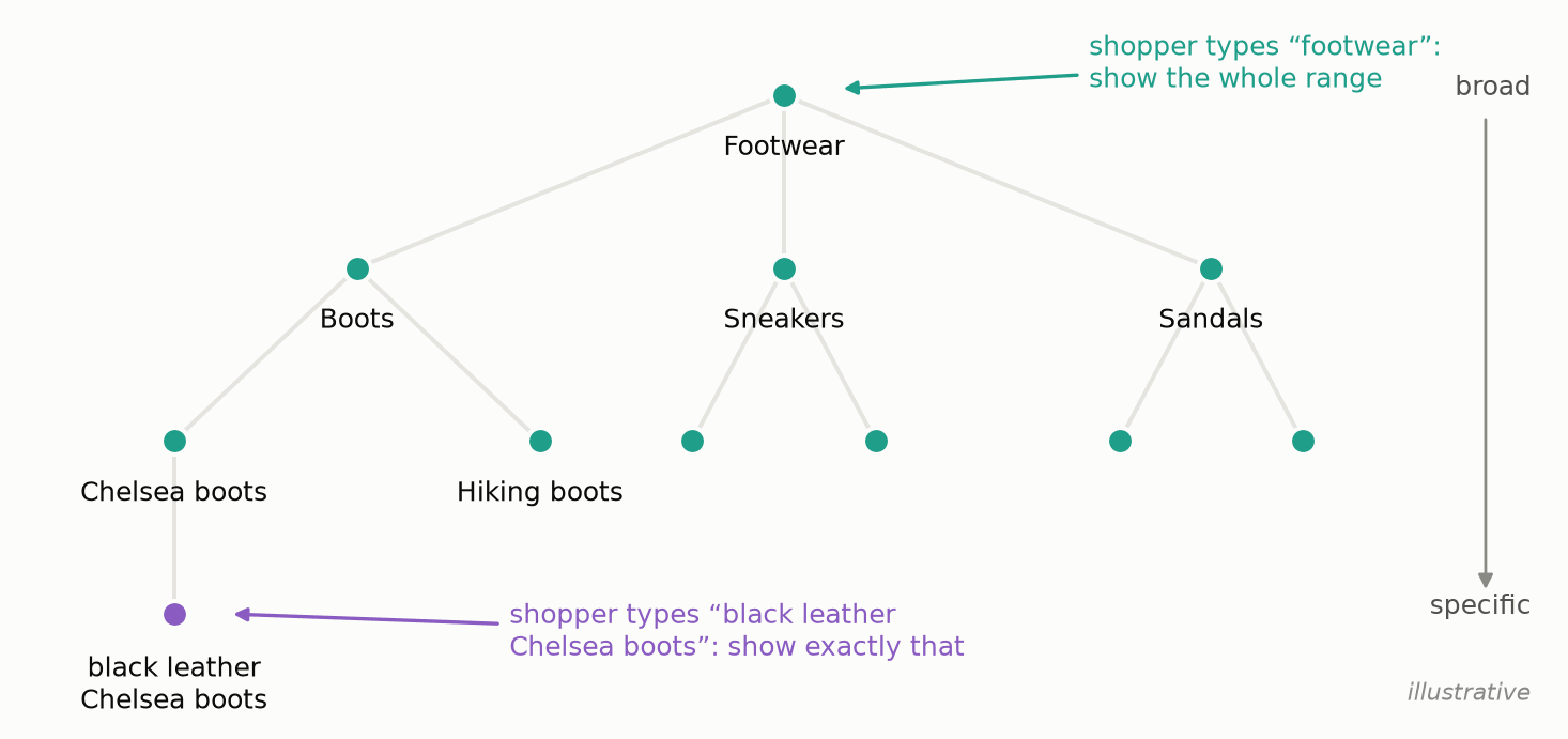A product hierarchy, broad at the top and specific at the bottom. A good search should know which level a query is aiming at.

Hyperbolic embedding models promise exactly that. An embedding is the list of numbers (a vector) that a model produces to represent a piece of text or an image, so that similar things get similar vectors. A hyperbolic model places those vectors in a curved space rather than a flat one, and in that space how general or specific something is becomes part of the vector itself. In practice it costs one extra number: the model we tested produces 513 numbers where its flat counterpart, OpenAI’s CLIP,^[1] produces 512. The first number works as a built-in specificity score: it rises from “vehicle” to “a red car” to "a red car on a city street". Below we’ll see where it comes from.

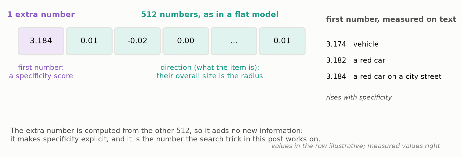One extra number up front, the height, acts as a built-in specificity score. The other 512 work as they do in a flat model.

Vector databases build their indexes around a handful of metrics: straight-line distance, inner product, cosine, and a few others for special data types. None of the mainstream ones we checked offers hyperbolic distance as a built-in index metric; some can compute it in a separate scoring or rerank step.

You don’t need a dedicated hyperbolic metric or a separate step. With one number flipped, a database’s ordinary inner-product search ranks by the exact hyperbolic score, a trick HypRAG’s authors^[2] already use (more below). What we add is the second step: one subtraction at ingest that lets those vectors survive the shortcuts real indexes take: the approximate part of approximate nearest neighbor (ANN), quantization and compression.

In this post we show that:

Hyperbolic search is inner-product search with one number flipped. Milvus can do it today.
One subtraction at ingest makes those vectors index well, with no rerank. It lifts recall on HNSW, IVF_FLAT and IVF_SQ8 (common index types, explained in part 2) and on Zilliz Cloud’s managed index.

We tested all of it on ImageNet,^[3] a standard dataset of about 1.28 million images in 1,000 categories, which are arranged in a hierarchy taken from WordNet (more on WordNet below).

Part 4 asks the other question: what the geometry does to the ranking itself.

Why hyperbolic?

Most embedding models, including CLIP, work in ordinary flat space (also called Euclidean), where distance is measured with a straight ruler. Flat space is good at "these two things are similar", but it has no built-in notion of "this is more general than that". For search, CLIP’s vectors are normalized to length 1, so “animal” cannot be a shorter vector than "a dog". If you need to know how broad something is, you usually store a separate taxonomy or train a separate classifier.

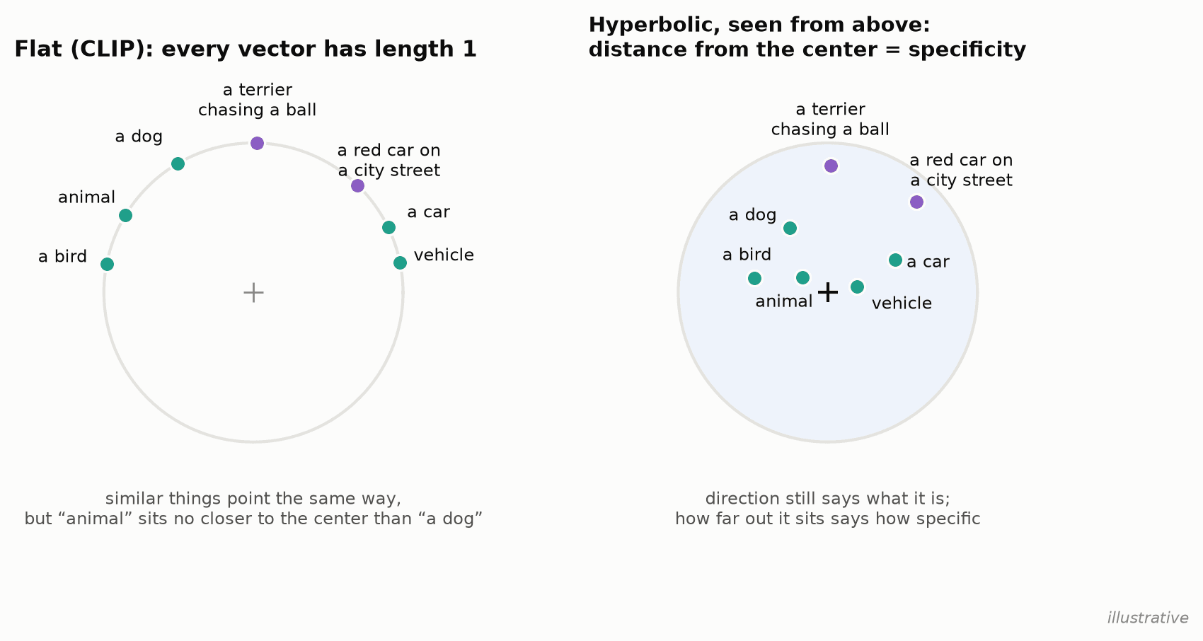In both spaces, direction says what an item is. Only in hyperbolic space does distance from the center also say how specific it is.

Flat space also runs out of room for trees. Every level of a hierarchy multiplies the number of items: one "animal", a handful of classes, hundreds of species, thousands of breeds. In flat space the room available grows far more slowly as you move outwards, so a flat model makes room for a big hierarchy by adding dimensions. In hyperbolic space, a curved space where the room available grows exponentially with distance from the center, a tree fits naturally.

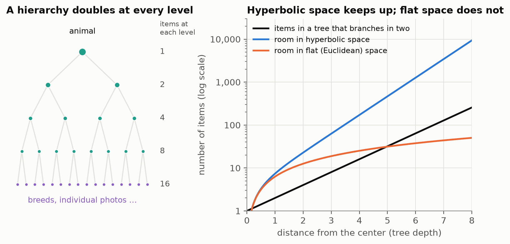Read the right-hand panel left to right as going deeper into a tree. The vertical axis is logarithmic, so the doubling tree (black) is a straight line. Hyperbolic room (blue) stays above it at every depth; flat room (orange) falls below it around depth 5, which is why a flat model has to add dimensions to fit a big hierarchy.

The classic evidence comes from WordNet,^[4] a large dictionary of English nouns arranged by “is a kind of” (a dog is a kind of animal). Nickel and Kiela (2017)^[5] embedded it in just 5 dimensions and asked each embedding to rank every noun as a candidate parent of a given noun. The hyperbolic embedding put the true parent at about 5th place on average. A flat embedding put it at about 3,500th, and even with 200 dimensions only reached about 1,160th. The hyperbolic embedding ranked the true parent over 700 times higher than a flat embedding of the same size, and still over 200 times higher than one with 40 times the dimensions. hyper³labs summarize this in The Geometry Mistake Behind Modern Embedding Models.

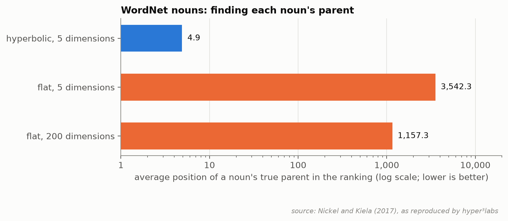Shorter bars are better: each is where the true parent landed in the ranking, on average. The axis is logarithmic, so each gridline is ten times the last. Five hyperbolic dimensions beat 200 flat ones by over 200 times.

The same idea now reaches text search. HypRAG, from Madhu et al. (2026),^[2] trains hyperbolic text encoders for retrieval-augmented generation (RAG), where a language model answers from passages a search returns. HyTE-FH is hyperbolic throughout; HyTE-H maps an existing flat encoder’s output into hyperbolic space. For HyTE-H they report gains of up to 29% over flat baselines in context and answer relevance on the RAGBench benchmark,^[6] using substantially smaller models than current state-of-the-art retrievers. Those are their results; everything we measure in this series uses an image-and-text model. Both HyTE models use the same Lorentz form as the model we tested, so the sign flip below applies to them exactly. Whether centering helps their vectors as much, we haven’t measured.

Broad concepts sit near the center

The model we used is Hyper3-CLIP V1 (hyper3labs/hyper3-clip-v1), a hyperbolic version of CLIP. CLIP is a vision-language model: it embeds text and images into the same space, so a text query can find matching images. hyper³labs recommend this checkpoint; their Hyper3-CLIP paper^[7] reports a sibling model, Hyper3-CLIP.

In this model, the more general a concept, the closer it sits to the center of the space. The distance from the center is called the radius, and we measured it for a range of phrases:

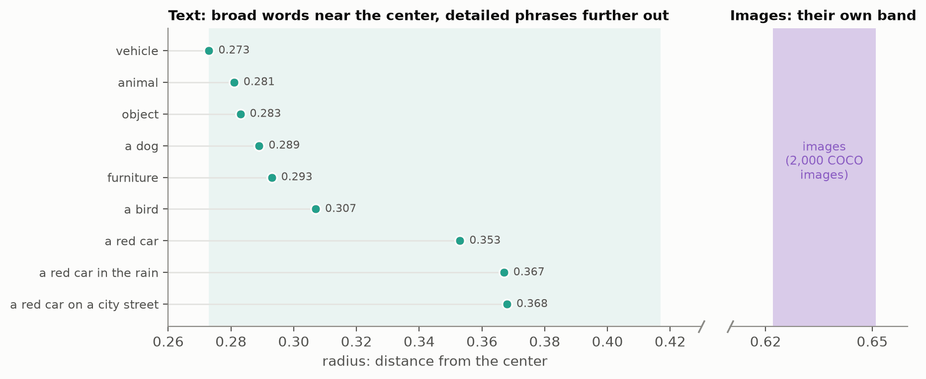Each dot is one phrase's distance from the center; further right is further out. Broad words sit left and detailed phrases right, with no labels supplied. Images (right panel, on a broken axis) sit in a band of their own beyond any text, so compare text with text and images with images.

Nobody labeled these; the order comes directly from the vectors. For an application, the radius is a useful signal in its own right: a way to tell a broad query from a specific one. hyper³labs’ post also shows, on handwritten digits, that ambiguous items tend to sit closer to the center than clear, typical ones, so the radius can flag those too.

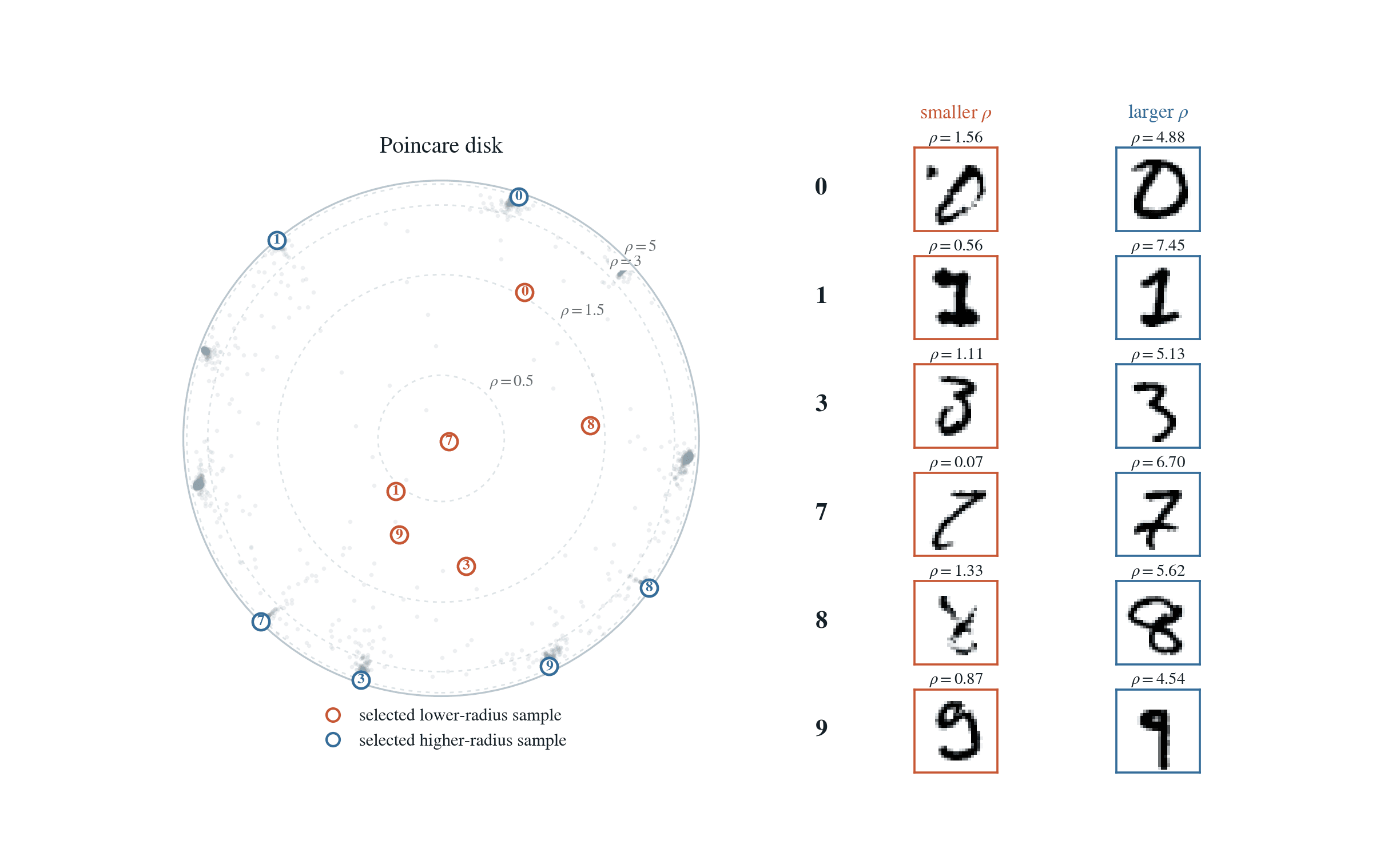Each row pairs two handwritten examples of the same digit: the orange box sits near the center, the blue one near the edge. The near-center digits are the scrawly, ambiguous ones. This is hyper³labs' figure, from their own handwritten-digit experiment, not from Hyper3-CLIP. Its ρ is a hyperbolic distance on a different scale, so don't compare it with our radii.

Source: hyper³labs.

Images sit in a band of their own, further out than any text (radius 0.62 to 0.65, against 0.27 to 0.42 for text), so compare text with text and images with images: an image is not “more specific” than a detailed caption just because it sits further out.

The space these vectors live in is called the Lorentz hyperboloid: picture a bowl-shaped surface, with its center (the origin) at the bottom. The most general concepts sit closest to it, and more specific ones sit further up the sides. The first of the 513 numbers is the point’s height up the bowl,^[8] and it rises with the radius. That is why it works as a specificity score. The other 512, the spatial coordinates, say which direction the point lies in, and their overall size is the radius.

Where does the minus sign in hyperbolic math come from? Each geometry measures closeness with its own inner product. CLIP’s vectors lie on a sphere: under the ordinary inner product, every one satisfies $x \cdot x = 1$ , and the distance between two of them along the sphere is the angle $\arccos(x \cdot y)$ . The hyperboloid is built the same way with one change: its inner product, the Lorentz inner product, subtracts the height’s contribution instead of adding it. Every point satisfies $\langle x, x \rangle_L = -10$ in this model, and distance along the bowl comes from $\langle x, y \rangle_L$ just as the sphere’s comes from $x \cdot y$ . That minus sign, with the constant now negative, turns a sphere, which curves back on itself and has limited room, into a bowl that opens outwards, with room growing exponentially as you move from the center. In geometry, the sphere is positively curved and the bowl negatively curved; “hyperbolic” means negatively curved.

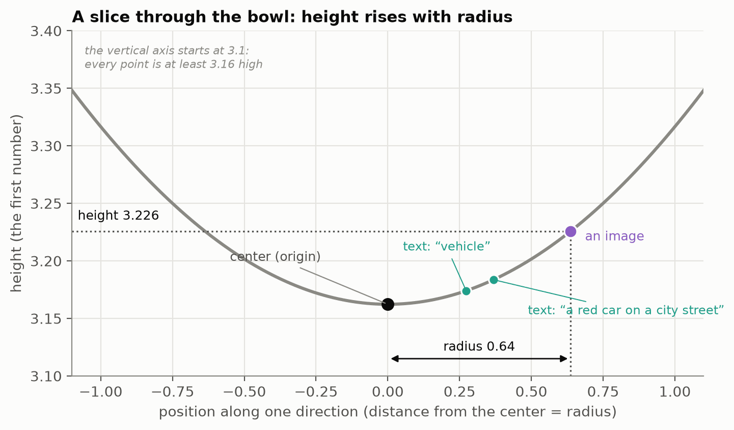The curve is the bowl seen side-on: move away from the center in any direction (horizontal axis) and the height, the first number, rises (vertical axis). The vertical axis starts at 3.1, which exaggerates the curve; every point is at least 3.16 high, which is why raw heights all sit around 3.2.

The math: why the height follows from the other 512

A point is $x = (x_0, \bar{x})$ : height $x_0$ and the 512 spatial coordinates $\bar{x}$ . Every point on the hyperboloid of curvature $-c$ satisfies

$\langle x, x \rangle_L = -x_0^2 + \lVert \bar{x} \rVert^2 = -\frac{1}{c} \quad\Longrightarrow\quad x_0 = \sqrt{\tfrac{1}{c} + \lVert \bar{x} \rVert^2}$

so the height is fixed by the radius $\lVert \bar{x} \rVert$ . For Hyper3-CLIP V1, $c = 0.1$ , so the lowest possible height, at the center, is $\sqrt{10} \approx 3.162$ . On real embeddings, $\langle x, x \rangle_L = -10.00000$ for text and images alike, and recomputing $x_0$ from the other 512 numbers matches the stored value to within $4.8 \times 10^{-7}$ .

A hyperbolic model judges closeness with the Lorentz inner product, minus sign included. A vector database offers the ordinary inner product, cosine and straight-line distance metrics, and none of them has that minus sign. What do you do?

Hyperbolic search is inner-product search

Vector search usually ranks results with one of three metrics: L2 (straight-line distance), inner product (IP: multiply the two vectors number by number and add the results up) and cosine (the angle between them). None of these is hyperbolic distance, so at first glance it looks as if you must either search hyperbolic vectors with the wrong metric, or give up the geometry.

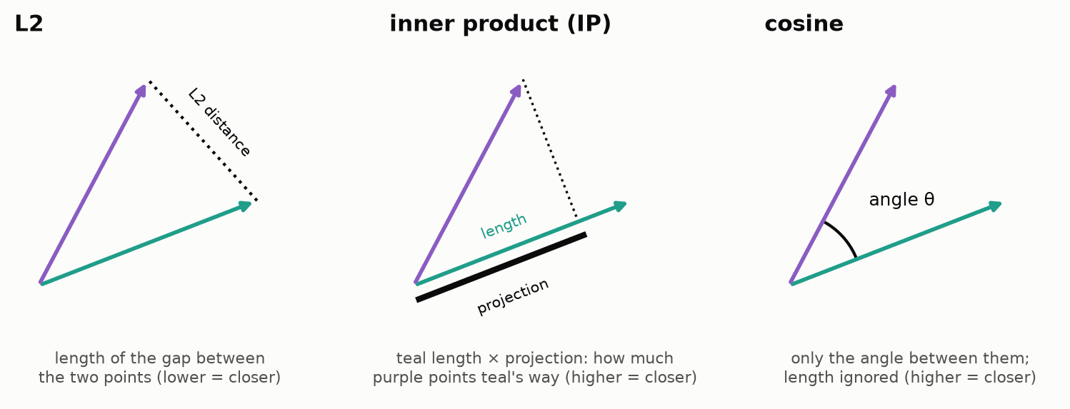The three metrics vector databases offer. Lower is closer for L2; higher is closer for inner product and cosine. Inner product is the one the sign flip turns into the hyperbolic score.

Hyperbolic models score two points with the Lorentz inner product, the ordinary inner product with the height’s contribution subtracted rather than added. Hyperbolic distance goes down whenever that score goes up, so ranking by one is exactly the same as ranking by the other.

That means you can:

store the vector exactly as the model produced it
flip the sign of the query’s height (its first number)
search with plain, unnormalized inner product

The inner product the database computes is then exactly the Lorentz score, and its top-k (the k best matches) matches the hyperbolic top-k.

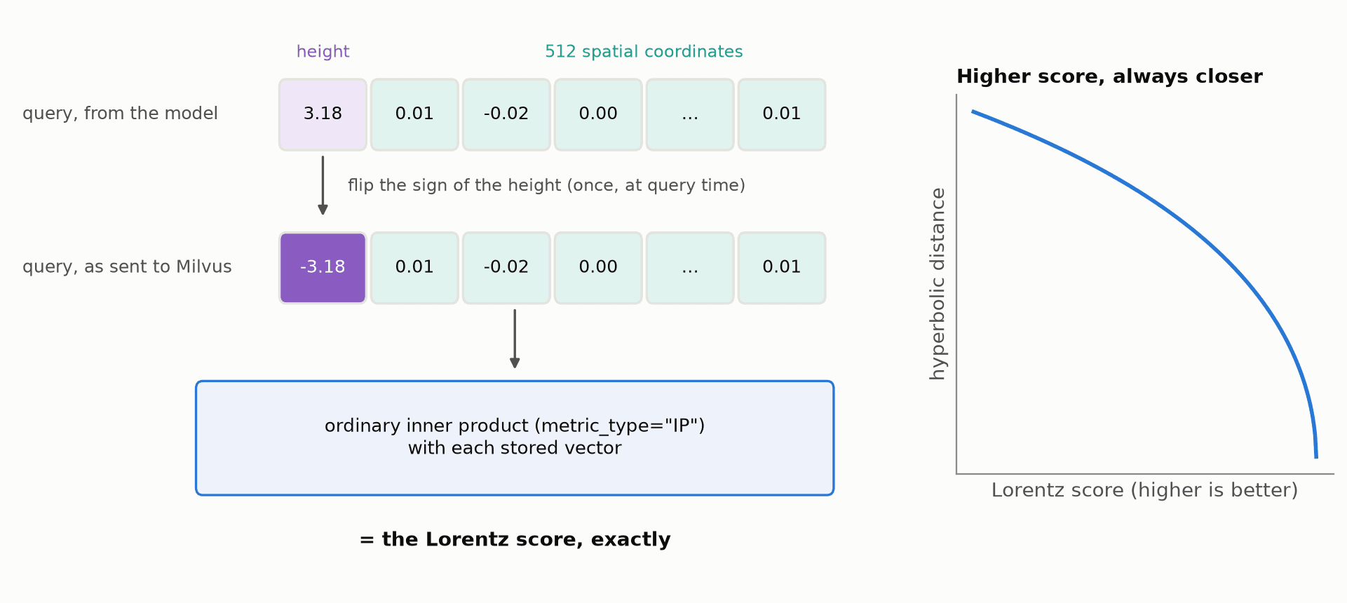Left: the only change is the sign of the query's first number; the database does an ordinary inner product. Right: hyperbolic distance falls whenever the Lorentz score rises, so sorting by highest score is the same as sorting by nearest.

q = np.array(emb, dtype=np.float32, copy=True)   # the query vector from the model
q[:, 0] *= -1.0                                  # flip the sign of the height
scores = docs @ q.T                              # = Lorentz inner product

We checked this against the model’s own scoring function on real embeddings. The largest difference was $3.9 \times 10^{-14}$ , which is floating-point rounding: more than ten billion times smaller than the typical gap between the top two results (0.0008). The order matched the order by hyperbolic distance exactly. This is not an approximation that happens to work. It is the same number.

We are not the first to use this reduction. In HypRAG (2026),^[2] Madhu et al. turn hyperbolic retrieval into inner-product search the same way, flipping the sign on the stored documents instead of the query; either side gives the same ranking. They indexed their hyperbolic text model, HyTE-FH, with Faiss’s HNSW index on 100,000 MS MARCO passages,^[9] and report that it reached a recall@10 of 0.906 with the sign flip alone. Their model, data and index settings differ from ours, so that figure isn’t comparable with the ones below. The next step, centering, is the novel part.

The math, for the curious

A point is $x = (x_0, \bar{x})$ , with height $x_0$ and spatial coordinates $\bar{x}$ . For curvature $-c$ (here $c = 0.1$ ):

$\langle x,y \rangle_L = -x_0 y_0 + \bar{x} \cdot \bar{y}, \qquad d(x,y) = \frac{\mathrm{arcosh}\left(-c \thinspace \langle x,y \rangle_L\right)}{\sqrt{c}}$

$\mathrm{arcosh}$ always increases, and its argument carries a minus sign, so the distance $d$ always falls as $\langle x,y \rangle_L$ rises. Negating $x_0$ in the query turns a plain dot product into $\langle x,y \rangle_L$ .

Center the height

The sign flip makes plain inner product return the exact hyperbolic ranking. On its own, though, it doesn’t make that search fast. Centering is the second, separate step that makes the exact search survive the optimizations that real indexes use for efficiency.

The problem: one number dwarfs the rest

Most vector search deployments use an approximate nearest neighbor (ANN) index, a data structure that finds nearly all of the best matches without comparing the query against every stored vector. Many also compress vectors to save memory. Both work by approximating the stored vectors, and hyperbolic vectors are hard to approximate out of the box.

Every vector in the corpus has a height of about 3.23, while each spatial coordinate is around ±0.02, over 100 times smaller. Here are the first 32 of the 513 numbers for one ImageNet image, a miniature schnauzer. The chart labels the height $x_0$ , and its lower panel shows the fix we come to below, which subtracts the corpus average height $m$ :

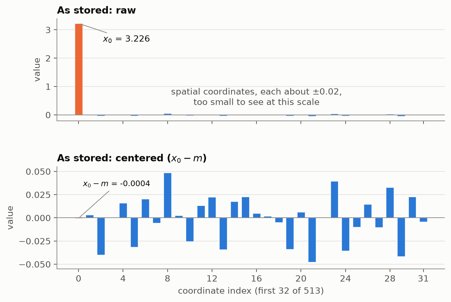The same vector twice, on very different vertical scales. Top: on a scale set by the height (orange), the 512 numbers that tell images apart are invisible. Bottom: centered, the height drops to almost zero and the axis rescales to show them.

As a result, almost every score is a large, nearly constant amount (about 10 in size) plus a tiny part that actually tells results apart. Across about 1.28 million images, the typical gap between the first and second result is 0.0008: under 0.01% of the score. An index or compression scheme spends its accuracy on the large common part and loses the part that matters.

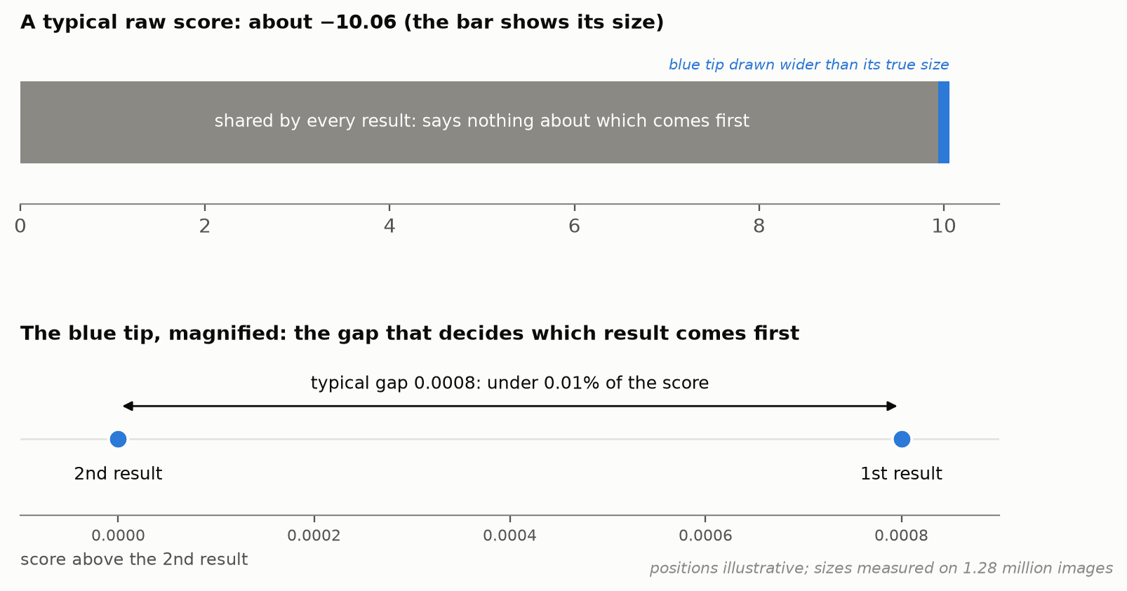Top: a raw score drawn to scale. The gray part is shared by every result, so it says nothing about the order. Bottom: the blue tip blown up to its own scale; the gap between first and second place is all that decides the ranking. Indexes and compression spend their precision on the gray bar, not the tip.

Why centering

We set ourselves a constraint: the database’s own inner-product search should return the hyperbolic top 10 directly. None of the mainstream databases we checked has a hyperbolic metric, and a custom scoring or rerank step needs extra fields, client code or engine-specific features. So a fix has to do three things at once:

keep the ranking exactly hyperbolic under plain inner product,
need nothing at query time beyond the sign flip, and
take the large shared part out of the stored vectors.

We measure success with recall@10: the share of the true 10 nearest neighbors that a search actually returns (1.0 means it found all of them). Here are the options:

option	ranking exactly hyperbolic?	indexes well?	needs a rerank?
store raw, flip the query’s sign	yes	no: recall@10 of 0.853 to 0.989, depending on the index	no
drop the height, or normalize and search by cosine	no: a cosine search reaches a recall@10 of only 0.745	yes: it’s ordinary cosine search	yes, to restore the order
center documents only, flip the query’s sign	yes	yes	no
shortlist by cosine, then rerank exactly (Strategy B in part 2)	yes, after the rerank	yes	yes

The fix is one subtraction. Compute $m$ , the average height over your corpus, once. Subtract it from the height of every stored document. Leave queries alone.

m = float(corpus[:, 0].mean())         # once, at ingest
docs = corpus.copy(); docs[:, 0] -= m  # documents only, never queries

Subtracting the same constant from every document’s height adds the same amount to every score a query produces: the query’s height times $m$ . The ranking is still exactly the hyperbolic ranking. Any constant would keep the ranking exact; we use the mean because it leaves the stored heights as close to zero as possible (within about 0.003 of zero).

The math: why the ranking is unchanged

Store each document as $(y_0 - m, \bar{y})$ and send the query as $(-x_0, \bar{x})$ . The inner product the database computes is

$-x_0 (y_0 - m) + \bar{x} \cdot \bar{y} = \langle x, y \rangle_L + x_0 m$

$x_0 m$ is the same for every document a query scores, so the ranking is exactly the Lorentz ranking; subtract $x_0 m$ from a returned score to recover the Lorentz score.

Why it should work

Floating-point numbers and quantizers keep precision relative to the size of the value they store. Centering shrinks the stored height from about 3.23 to within about 0.003 of zero, while keeping all of the variation between documents that carries the ranking. That variation becomes large relative to the stored number, so it survives rounding.

Compression makes this easy to see. Storing vectors as fp16 (16-bit floating point numbers, half the memory of the usual 32-bit fp32) keeps only about three significant digits. In a sample of 2,000 COCO images^[10] we measured, the heights all fell between about 3.223 and 3.229 (the ImageNet average, 3.2263, sits inside that band), and fp16 rounds every one of them onto at most four values, so images with different heights end up tied. Centered, the same spread sits around zero, where fp16 has over 13,000 values to choose from and every image keeps its own height.

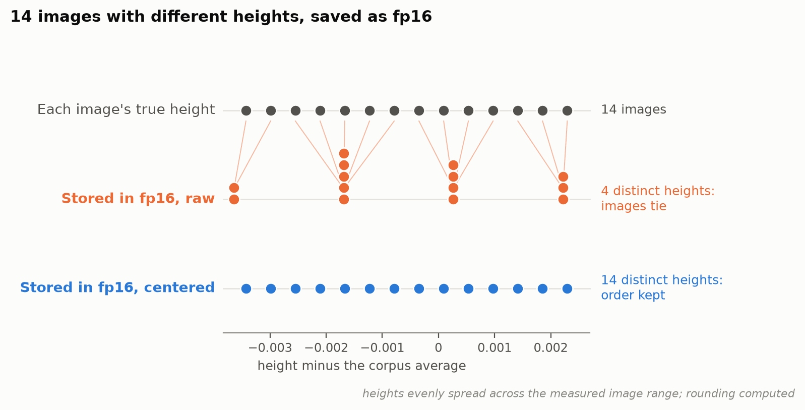Follow each image down from its true height (top row) to the height fp16 stores. Raw (orange), the 14 images round onto 4 values and stack up, so images in the same pile tie and their order is lost. Centered (blue), every image keeps its own height. The heights are evenly spread across the measured image range; the rounding is computed.

The same holds at full precision. In a brute-force search at 32-bit precision, with no approximation at all, the largest score error falls from $7.8 \times 10^{-6}$ to $1.1 \times 10^{-7}$ : about 70 times smaller, because the arithmetic no longer carries the large shared part through every score.

Indexes are affected in the same way. Graph and cluster indexes are built from similarities between stored vectors. Raw, those similarities are almost entirely the shared part; centered, they are dominated by the part that differs between documents.

That explanation makes predictions we can check. Centering should help wherever the approximation treats all 513 numbers on one scale: graph indexes (HNSW), cluster indexes (IVF), and fp16 storage. It should not help the compression step where each number already gets its own range, as in Milvus’s 8-bit IVF_SQ8 quantizer. Both predictions hold: with every cluster searched, so that only the compression is left to matter, IVF_SQ8 reaches a recall@10 of 0.978 raw or centered. One result it doesn’t predict: product quantization (IVF_PQ) fails with or without centering, and centering makes it slightly worse (recall 0.115 raw, 0.096 centered), so don’t use this approach on a PQ index. Part 2 has the details.

The evidence, with no rerank

Every figure below is the database’s own inner-product search with the sign-flipped query. Nothing re-scores or reorders the results afterwards. The only application-side work is subtracting $m$ once at ingest and flipping the sign of one number per query.

It matches the rerank design. On Milvus with HNSW (ef=128), centered vectors reach a recall@10 of 0.996 in a single search. Strategy B, which reranks a 200-candidate shortlist, also reaches 0.996; the confidence intervals overlap.
It improves recall on graph and cluster indexes. On Milvus, centering lifts IVF_FLAT’s recall@10 from 0.900 to 0.990, ten times fewer misses, and HNSW (ef=64) from 0.974 to 0.989 (part 2 has the index-by-index results).
It replaces a big shortlist on a managed index to get the same recall. On Zilliz Cloud, centered vectors reach a recall@10 of 0.982 in one request. Raw vectors need a 1,000-result shortlist and a rerank step to reach 0.980 (part 3).
The database really is computing the hyperbolic score. Once the constant offset is removed, the scores that Milvus and Zilliz Cloud return are typically within 0.000011 of the exact Lorentz score, about ten times smaller than the typical gap between the 10th and 11th results.
It survives compression. In a simulation that stores vectors as fp16 and searches them exhaustively, raw vectors reach a recall@10 of 0.607 and centered vectors 0.997.

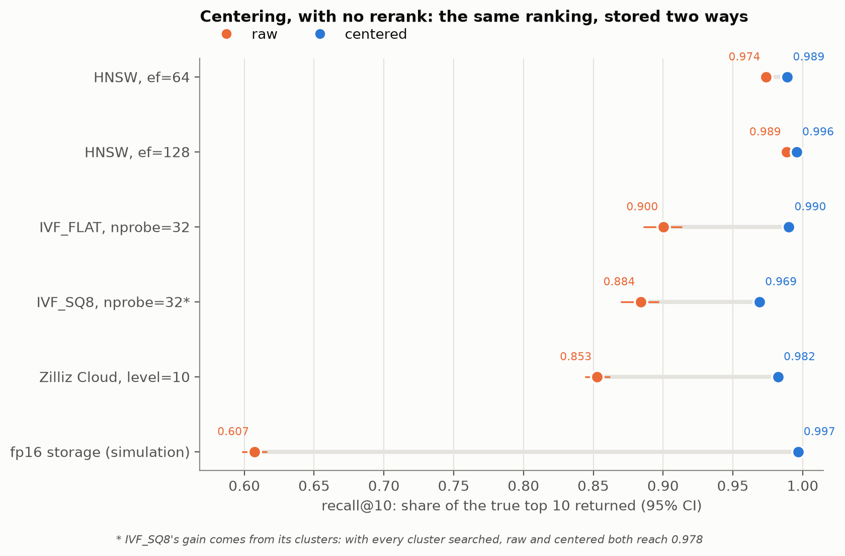Each row is one index or storage setting. Orange is raw, blue is centered, and further right means more of the true top 10 found; the gray bar is what centering gains. Centered is at or above raw in every row, and gains most where the approximation is coarsest: IVF clusters, the managed index and fp16.

What we are not claiming

That centering helps every model equally. The sign flip is exact for any model in this Lorentz form. Centering’s benefit is measured on one model, Hyper3-CLIP V1, and one image collection.

Takeaway

You don’t need a hyperbolic metric. Flip the sign of the query’s height, search with plain inner product, and you get the exact hyperbolic ranking.
Center your documents, not your queries. Subtract the average height at ingest and the same vectors survive indexing and compression, with no rerank.
Then ask what the geometry buys you. Part 4 compares Hyper3-CLIP V1 with CLIP, and with its own cosine scorer.

Part 2 turns this into a Milvus deployment, with index-by-index recall.